Use label_number() to force decimal display of numbers (i.e. don't use
scientific notation). label_comma() is a special case
that inserts a comma every three digits.
Usage
label_number(
  accuracy = NULL,
  scale = 1,
  prefix = "",
  suffix = "",
  big.mark = NULL,
  decimal.mark = NULL,
  style_positive = NULL,
  style_negative = NULL,
  scale_cut = NULL,
  trim = TRUE,
  ...
)

label_comma(
  accuracy = NULL,
  scale = 1,
  prefix = "",
  suffix = "",
  big.mark = ",",
  decimal.mark = ".",
  trim = TRUE,
  digits,
  ...
)
Arguments
- accuracy
A number to round to. Use (e.g.)
0.01to show 2 decimal places of precision. IfNULL, the default, uses a heuristic that should ensure breaks have the minimum number of digits needed to show the difference between adjacent values.Applied to rescaled data.
- scale
A scaling factor:
xwill be multiplied byscalebefore formatting. This is useful if the underlying data is very small or very large.- prefix
Additional text to display before the number. The suffix is applied to absolute value before
style_positiveandstyle_negativeare processed so thatprefix = "$"will yield (e.g.)-$1and($1).- suffix
Additional text to display after the number.
- big.mark
Character used between every 3 digits to separate thousands. The default (
NULL) retrieves the setting from the number options.- decimal.mark
The character to be used to indicate the numeric decimal point. The default (
NULL) retrieves the setting from the number options.- style_positive
A string that determines the style of positive numbers:
"none"(the default): no change, e.g.1."plus": preceded by+, e.g.+1."space": preceded by a Unicode "figure space", i.e., a space equally as wide as a number or+. Compared to"none", adding a figure space can ensure numbers remain properly aligned when they are left- or right-justified.
The default (
NULL) retrieves the setting from the number options.- style_negative
A string that determines the style of negative numbers:
"hyphen"(the default): preceded by a standard hyphen-, e.g.-1."minus", uses a proper Unicode minus symbol. This is a typographical nicety that ensures-aligns with the horizontal bar of the the horizontal bar of+."parens", wrapped in parentheses, e.g.(1).
The default (
NULL) retrieves the setting from the number options.- scale_cut
Named numeric vector that allows you to rescale large (or small) numbers and add a prefix. Built-in helpers include:
cut_short_scale(): [10^3, 10^6) = K, [10^6, 10^9) = M, [10^9, 10^12) = B, [10^12, Inf) = T.cut_long_scale(): [10^3, 10^6) = K, [10^6, 10^12) = M, [10^12, 10^18) = B, [10^18, Inf) = T.cut_si(unit): uses standard SI units.
If you supply a vector
c(a = 100, b = 1000), absolute values in the range[0, 100)will not be rescaled, absolute values in the range[100, 1000)will be divided by 100 and given the suffix "a", and absolute values in the range[1000, Inf)will be divided by 1000 and given the suffix "b". If the division creates an irrational value (or one with many digits), the cut value below will be tried to see if it improves the look of the final label.- trim
Logical, if
FALSE, values are right-justified to a common width (seebase::format()).- ...
Other arguments passed on to
base::format().- digits
![[Deprecated]](figures/lifecycle-deprecated.svg) Use
Use accuracyinstead.
Value
All label_() functions return a "labelling" function, i.e. a function that
takes a vector x and returns a character vector of length(x) giving a
label for each input value.
Labelling functions are designed to be used with the labels argument of
ggplot2 scales. The examples demonstrate their use with x scales, but
they work similarly for all scales, including those that generate legends
rather than axes.
Examples
demo_continuous(c(-1e6, 1e6))
#> scale_x_continuous()
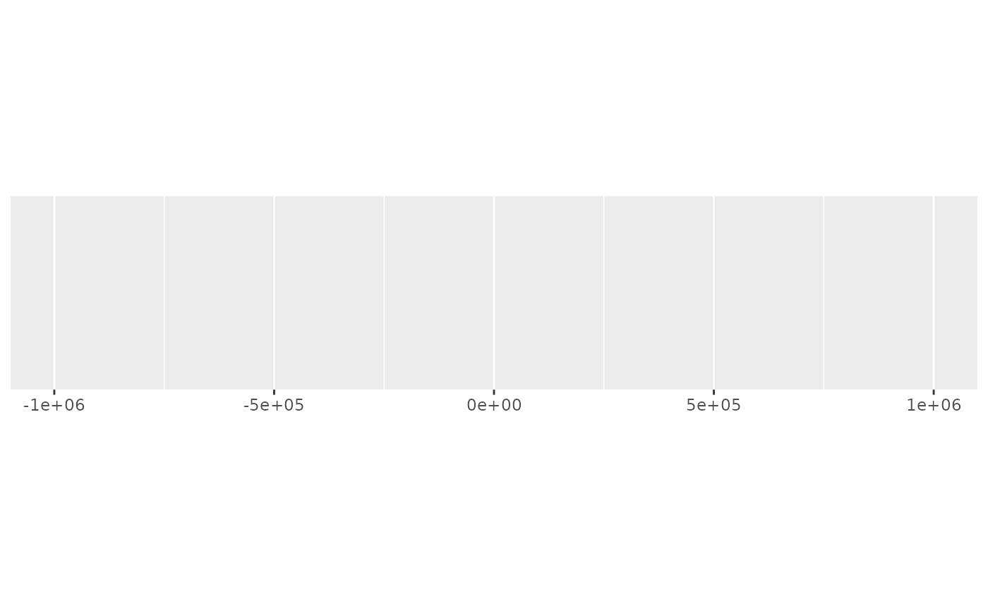 demo_continuous(c(-1e6, 1e6), labels = label_number())
#> scale_x_continuous(labels = label_number())
demo_continuous(c(-1e6, 1e6), labels = label_number())
#> scale_x_continuous(labels = label_number())
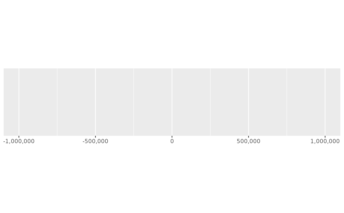
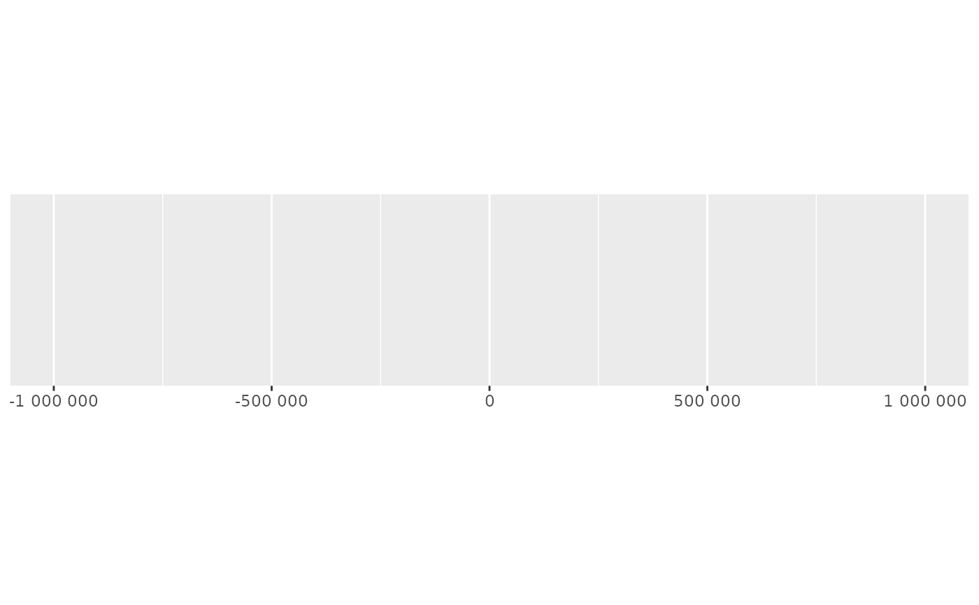 demo_continuous(c(-1e6, 1e6), labels = label_comma())
#> scale_x_continuous(labels = label_comma())
demo_continuous(c(-1e6, 1e6), labels = label_comma())
#> scale_x_continuous(labels = label_comma())
 # Use scale to rescale very small or large numbers to generate
# more readable labels
demo_continuous(c(0, 1e6), labels = label_number())
#> scale_x_continuous(labels = label_number())
# Use scale to rescale very small or large numbers to generate
# more readable labels
demo_continuous(c(0, 1e6), labels = label_number())
#> scale_x_continuous(labels = label_number())
 demo_continuous(c(0, 1e6), labels = label_number(scale = 1 / 1e3))
#> scale_x_continuous(labels = label_number(scale = 1/1000))
demo_continuous(c(0, 1e6), labels = label_number(scale = 1 / 1e3))
#> scale_x_continuous(labels = label_number(scale = 1/1000))
 demo_continuous(c(0, 1e-6), labels = label_number())
#> scale_x_continuous(labels = label_number())
demo_continuous(c(0, 1e-6), labels = label_number())
#> scale_x_continuous(labels = label_number())
 demo_continuous(c(0, 1e-6), labels = label_number(scale = 1e6))
#> scale_x_continuous(labels = label_number(scale = 1e+06))
demo_continuous(c(0, 1e-6), labels = label_number(scale = 1e6))
#> scale_x_continuous(labels = label_number(scale = 1e+06))
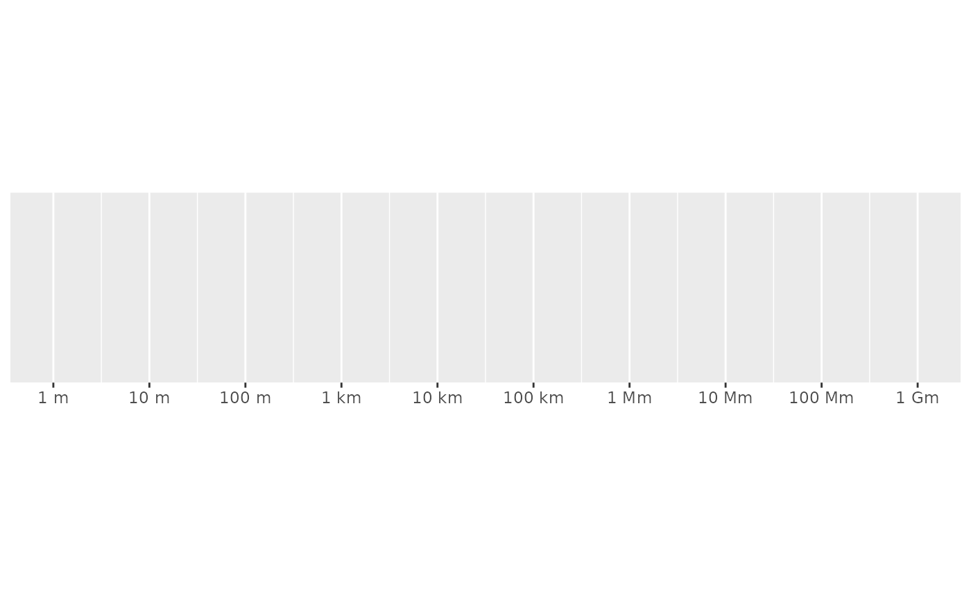
 #' Use scale_cut to automatically add prefixes for large/small numbers
demo_log10(
c(1, 1e9),
breaks = log_breaks(10),
labels = label_number(scale_cut = cut_short_scale())
)
#> scale_x_log10(breaks = log_breaks(10), labels = label_number(scale_cut = cut_short_scale()))
#' Use scale_cut to automatically add prefixes for large/small numbers
demo_log10(
c(1, 1e9),
breaks = log_breaks(10),
labels = label_number(scale_cut = cut_short_scale())
)
#> scale_x_log10(breaks = log_breaks(10), labels = label_number(scale_cut = cut_short_scale()))
 demo_log10(
c(1, 1e9),
breaks = log_breaks(10),
labels = label_number(scale_cut = cut_si("m"))
)
#> scale_x_log10(breaks = log_breaks(10), labels = label_number(scale_cut = cut_si("m")))
demo_log10(
c(1, 1e9),
breaks = log_breaks(10),
labels = label_number(scale_cut = cut_si("m"))
)
#> scale_x_log10(breaks = log_breaks(10), labels = label_number(scale_cut = cut_si("m")))
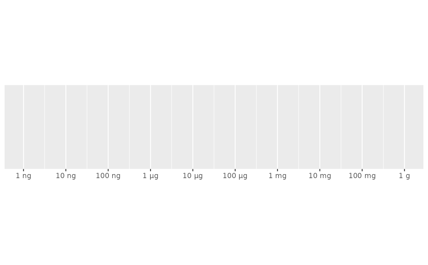
 demo_log10(
c(1e-9, 1),
breaks = log_breaks(10),
labels = label_number(scale_cut = cut_si("g"))
)
#> scale_x_log10(breaks = log_breaks(10), labels = label_number(scale_cut = cut_si("g")))
demo_log10(
c(1e-9, 1),
breaks = log_breaks(10),
labels = label_number(scale_cut = cut_si("g"))
)
#> scale_x_log10(breaks = log_breaks(10), labels = label_number(scale_cut = cut_si("g")))
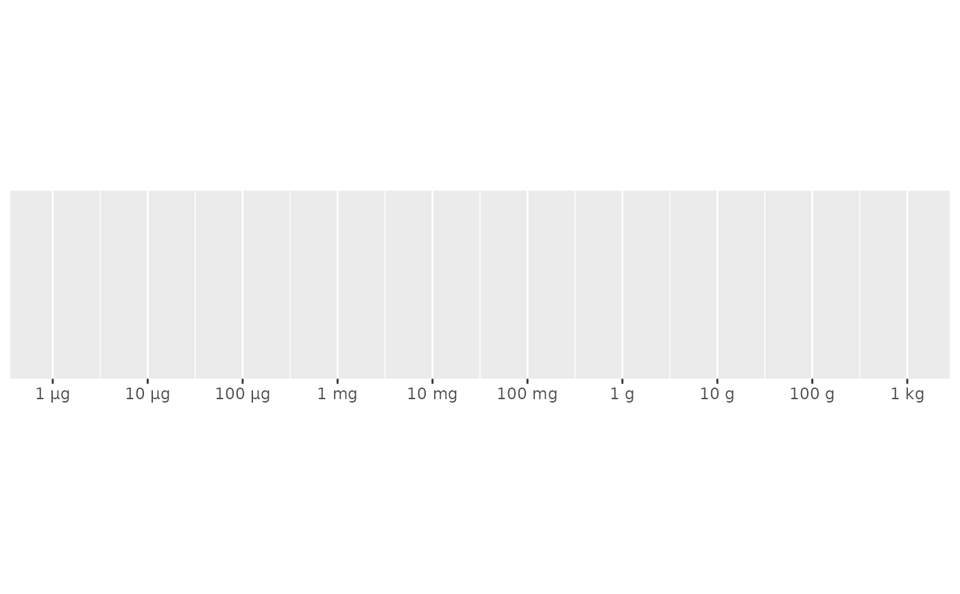
 # use scale and scale_cut when data already uses SI prefix
# for example, if data was stored in kg
demo_log10(
c(1e-9, 1),
breaks = log_breaks(10),
labels = label_number(scale_cut = cut_si("g"), scale = 1e3)
)
#> scale_x_log10(breaks = log_breaks(10), labels = label_number(scale_cut = cut_si("g"),
#> scale = 1000))
# use scale and scale_cut when data already uses SI prefix
# for example, if data was stored in kg
demo_log10(
c(1e-9, 1),
breaks = log_breaks(10),
labels = label_number(scale_cut = cut_si("g"), scale = 1e3)
)
#> scale_x_log10(breaks = log_breaks(10), labels = label_number(scale_cut = cut_si("g"),
#> scale = 1000))
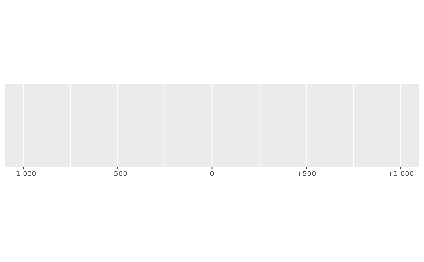
 #' # Use style arguments to vary the appearance of positive and negative numbers
demo_continuous(c(-1e3, 1e3), labels = label_number(
style_positive = "plus",
style_negative = "minus"
))
#> scale_x_continuous(labels = label_number(style_positive = "plus",
#> style_negative = "minus"))
#' # Use style arguments to vary the appearance of positive and negative numbers
demo_continuous(c(-1e3, 1e3), labels = label_number(
style_positive = "plus",
style_negative = "minus"
))
#> scale_x_continuous(labels = label_number(style_positive = "plus",
#> style_negative = "minus"))
 demo_continuous(c(-1e3, 1e3), labels = label_number(style_negative = "parens"))
#> scale_x_continuous(labels = label_number(style_negative = "parens"))
demo_continuous(c(-1e3, 1e3), labels = label_number(style_negative = "parens"))
#> scale_x_continuous(labels = label_number(style_negative = "parens"))
 # You can use prefix and suffix for other types of display
demo_continuous(c(32, 212), labels = label_number(suffix = "\u00b0F"))
#> scale_x_continuous(labels = label_number(suffix = "°F"))
# You can use prefix and suffix for other types of display
demo_continuous(c(32, 212), labels = label_number(suffix = "\u00b0F"))
#> scale_x_continuous(labels = label_number(suffix = "°F"))
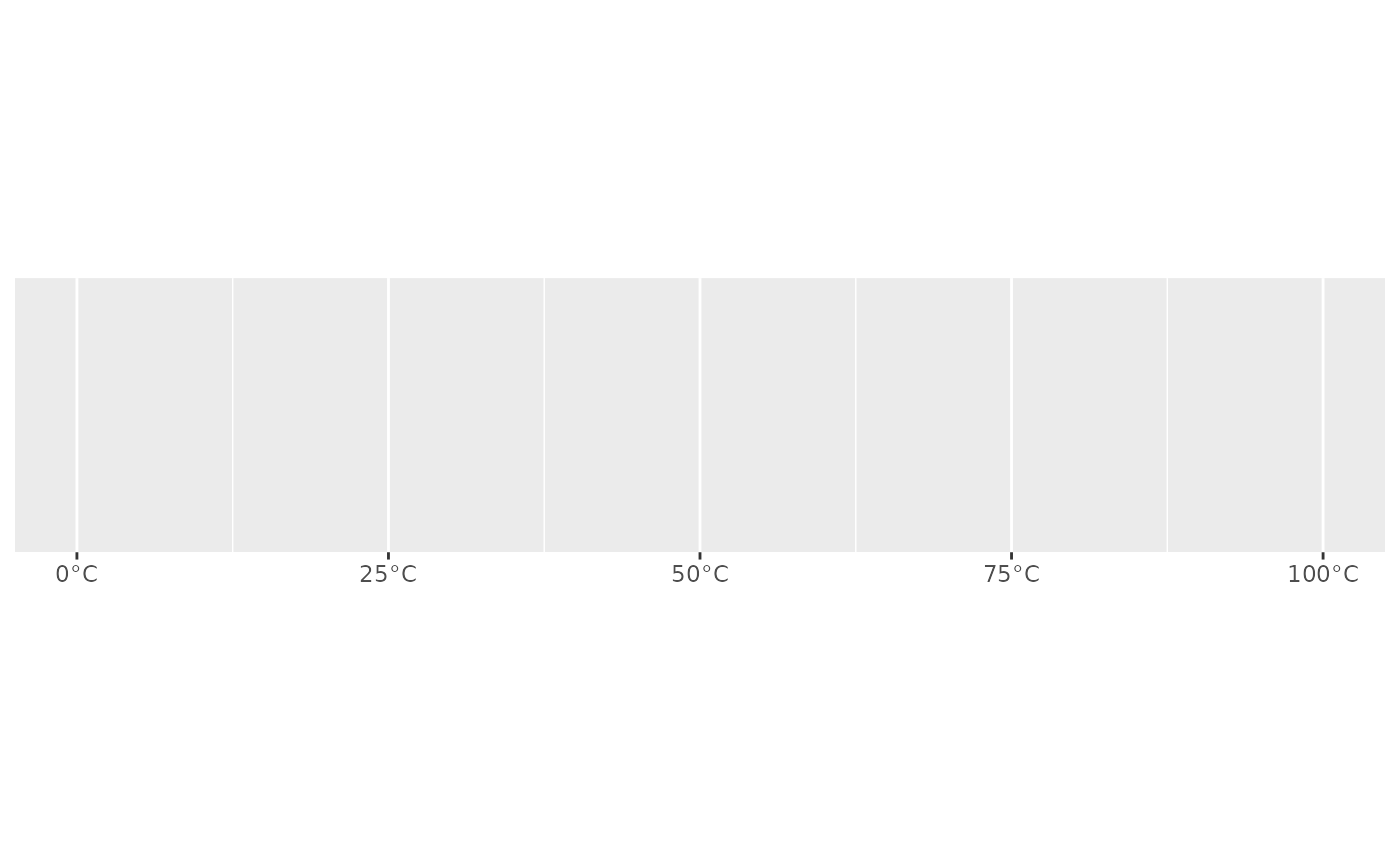
 demo_continuous(c(0, 100), labels = label_number(suffix = "\u00b0C"))
#> scale_x_continuous(labels = label_number(suffix = "°C"))
demo_continuous(c(0, 100), labels = label_number(suffix = "\u00b0C"))
#> scale_x_continuous(labels = label_number(suffix = "°C"))